Analysing the climate at spatial points for a given period
Source:vignettes/points-df-mat-sf.Rmd
points-df-mat-sf.RmdWith {easyclimate} you can easily download daily, monthly and annual climate data for a given set of points or polygons within Europe. To download and install the latest version of {easyclimate} from GitHub follow the instructions in https://github.com/VeruGHub/easyclimate
In this tutorial we will work through the basics of using easyclimate
with coordinate points. You can enter coordinates as a
data.frame, matrix, sf or
SpatVector object. At the end we will have a data frame
with climate variables for each point.
Example 1: Introducing coordinates as a data frame
First, specify longitude and latitude coordinates in a data frame
with the column names lon and lat. Here we are
simulating coordinates for three random sites in southern Spain:
library(easyclimate)
library(ggplot2)
library(dplyr)

coords <- data.frame(
  lon = rnorm(3, mean = -5.36, sd = 0.3),
  lat = rnorm(3, mean = 37.40, sd = 0.3)
  )

ggplot() +
  borders(regions = c("Spain", "Portugal", "France")) +
    geom_point(data = coords, aes(x = lon, y = lat)) +
  coord_fixed(xlim = c(-10, 2), ylim = c(36, 44), ratio = 1.3) +
    xlab("Longitude") +
    ylab("Latitude") +
  theme_bw()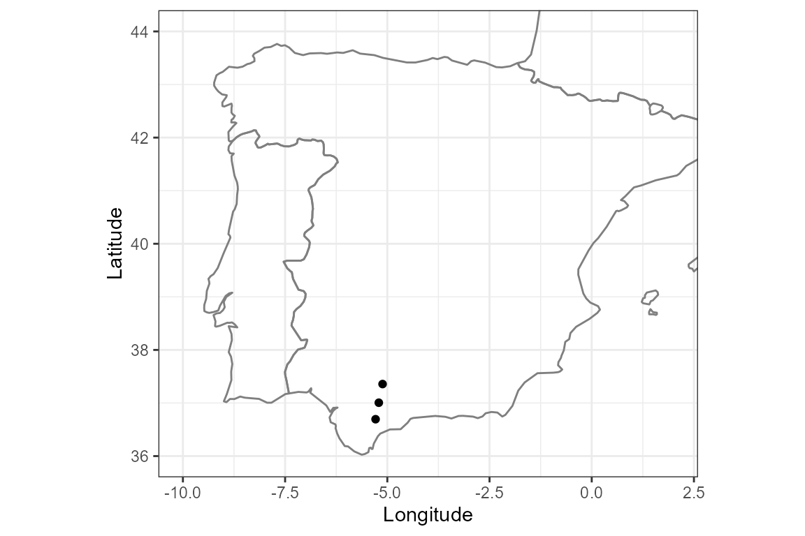
Now, download the climatic data for the selected locations. To get
daily data, all you have to do is use the function
get_daily_climate, specifying the period
(e.g. 2008-05-25 for a single day or 2008:2010
for several years), and the variables to be downloaded (precipitation
Prcp, minimum temperature Tmin or maximum
temperature Tmax).You can also use the function
get_monthly_climateand get_annual_climateto
download monthly and annual data, specifying the period
(e.g. 2008-05for a single month, 2008 for a
single year, or 2008:2010 for several years):
Sys.time() # to know how much time it takes to download
## [1] "2025-12-18 21:30:13 CET"

daily <- get_daily_climate( # daily data
  coords = coords,
  period = 2008:2010,
  climatic_var = c("Prcp", "Tmin", "Tmax")
  )

Sys.time()
## [1] "2025-12-18 21:34:40 CET"

kable(head(daily))| ID_coords | lon | lat | date | Prcp | Tmin | Tmax |
|---|---|---|---|---|---|---|
| 1 | -5.780013 | 37.39833 | 2008-01-01 | 6.95 | 3.62 | 14.24 |
| 1 | -5.780013 | 37.39833 | 2008-01-02 | 25.34 | 8.93 | 15.70 |
| 1 | -5.780013 | 37.39833 | 2008-01-03 | 4.12 | 8.15 | 14.49 |
| 1 | -5.780013 | 37.39833 | 2008-01-04 | 0.00 | 5.31 | 13.91 |
| 1 | -5.780013 | 37.39833 | 2008-01-05 | 0.00 | 5.76 | 14.45 |
| 1 | -5.780013 | 37.39833 | 2008-01-06 | 0.00 | 11.33 | 15.14 |
Sys.time()
## [1] "2025-12-18 21:34:40 CET"

monthly <- get_monthly_climate( # monthly data
  coords = coords,
  period = 2008:2010,
  climatic_var = c("Prcp", "Tmin", "Tavg", "Tmax")
  )

Sys.time()
## [1] "2025-12-18 21:35:04 CET"

kable(head(monthly))| ID_coords | lon | lat | date | Prcp | Tmin | Tavg | Tmax |
|---|---|---|---|---|---|---|---|
| 1 | -5.780013 | 37.39833 | 2008-01 | 47.50 | 6.80 | 12.01 | 17.21 |
| 1 | -5.780013 | 37.39833 | 2008-02 | 59.22 | 9.41 | 14.41 | 19.41 |
| 1 | -5.780013 | 37.39833 | 2008-03 | 14.89 | 8.13 | 14.80 | 21.48 |
| 1 | -5.780013 | 37.39833 | 2008-04 | 181.45 | 11.29 | 17.42 | 23.55 |
| 1 | -5.780013 | 37.39833 | 2008-05 | 51.06 | 13.47 | 19.05 | 24.62 |
| 1 | -5.780013 | 37.39833 | 2008-06 | 0.00 | 17.71 | 25.60 | 33.49 |
annual <- get_annual_climate( # annual data
  coords = coords,
  period = 2008:2010,
  climatic_var = c("Prcp", "Tmin", "Tavg", "Tmax")
  )

Sys.time()
## [1] "2025-12-18 21:35:14 CET"

kable(head(annual))| ID_coords | lon | lat | date | Prcp | Tmin | Tavg | Tmax |
|---|---|---|---|---|---|---|---|
| 1 | -5.780013 | 37.39833 | 2008 | 524.71 | 12.51 | 18.63 | 24.75 |
| 1 | -5.780013 | 37.39833 | 2009 | 609.27 | 13.22 | 19.43 | 25.65 |
| 1 | -5.780013 | 37.39833 | 2010 | 927.66 | 13.48 | 19.02 | 24.57 |
| 2 | -5.283405 | 37.58647 | 2008 | 491.54 | 10.85 | 17.81 | 24.77 |
| 2 | -5.283405 | 37.58647 | 2009 | NA | 11.74 | 18.71 | 25.68 |
| 2 | -5.283405 | 37.58647 | 2010 | 1046.42 | 12.12 | 18.23 | 24.34 |
Here we extract different components of the date:
library(lubridate)

daily <- daily |>
  mutate(
    date = as.Date(date),
    month = months(date),
    year = format(date, format = "%y")
  )

monthly <- monthly |>
  mutate(date = ym(date))
Finally, you can visualize the daily, monthly and annual climate results. For example, let’s plot the precipitation for one of the sites:
clim_daily_site1 <- daily |>
  filter(ID_coords == 1)

ggplot(clim_daily_site1) +
  geom_line(aes(x = date, y = Prcp), colour = "steelblue") +
  labs(x = "Date", y = "Daily precipitation (mm)") +
  theme_bw()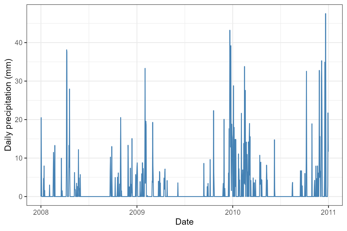
clim_monthly_site1 <- monthly |>
  filter(ID_coords == 1)

ggplot(clim_monthly_site1) +
  geom_line(aes(x = date, y = Prcp), colour = "steelblue") +
  labs(x = "Date", y = "Monthly precipitation (mm)") +
  theme_bw()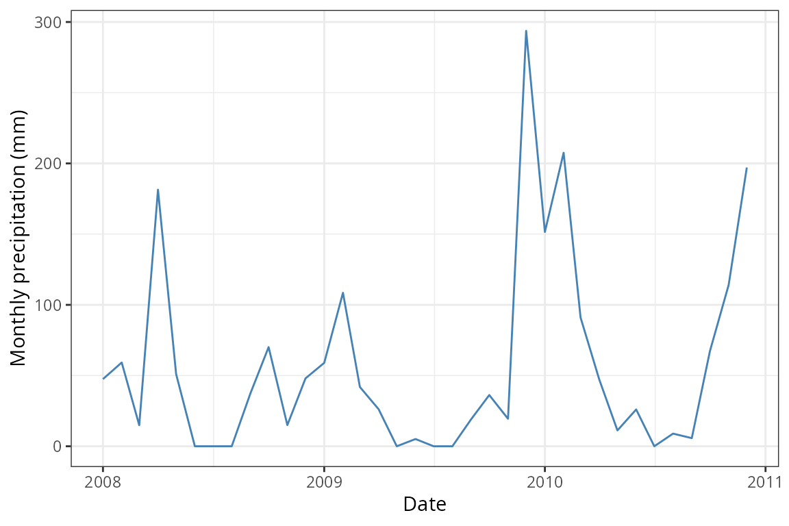
clim_annual_site1 <- annual |>
  filter(ID_coords == 1)

ggplot(clim_annual_site1) +
  geom_line(aes(x = date, y = Prcp), colour = "steelblue") +
  labs(x = "Date", y = "Annual precipitation (mm)") +
  scale_x_continuous(breaks = scales::breaks_width(1)) +
  theme_bw()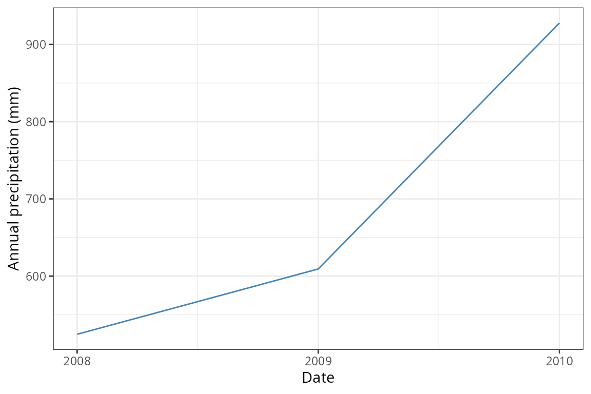
Or calculate the daily mean temperature and plot it against
tmin and tmax:
library(tidyr)

temp_long <- daily |>
  mutate(Tmean = (Tmin + Tmax) / 2) |>
  pivot_longer(
    cols = c("Tmin", "Tmax", "Tmean"),
    names_to = "temp_vars",
    values_to = "temp_values")

ggplot(temp_long, aes(x = factor(ID_coords), y = temp_values,
                      fill = temp_vars, color = temp_vars)) +
  geom_violin(size = 1, alpha = .7) +
    scale_fill_manual(values = c("#C54A52", "#FAFBC5", "#4B8AB8")) +
  scale_color_manual(values = c("#C54A52", "#FAFBC5", "#4B8AB8")) +
  ylab("Temperature (ºC)") + xlab("") +
  theme_bw()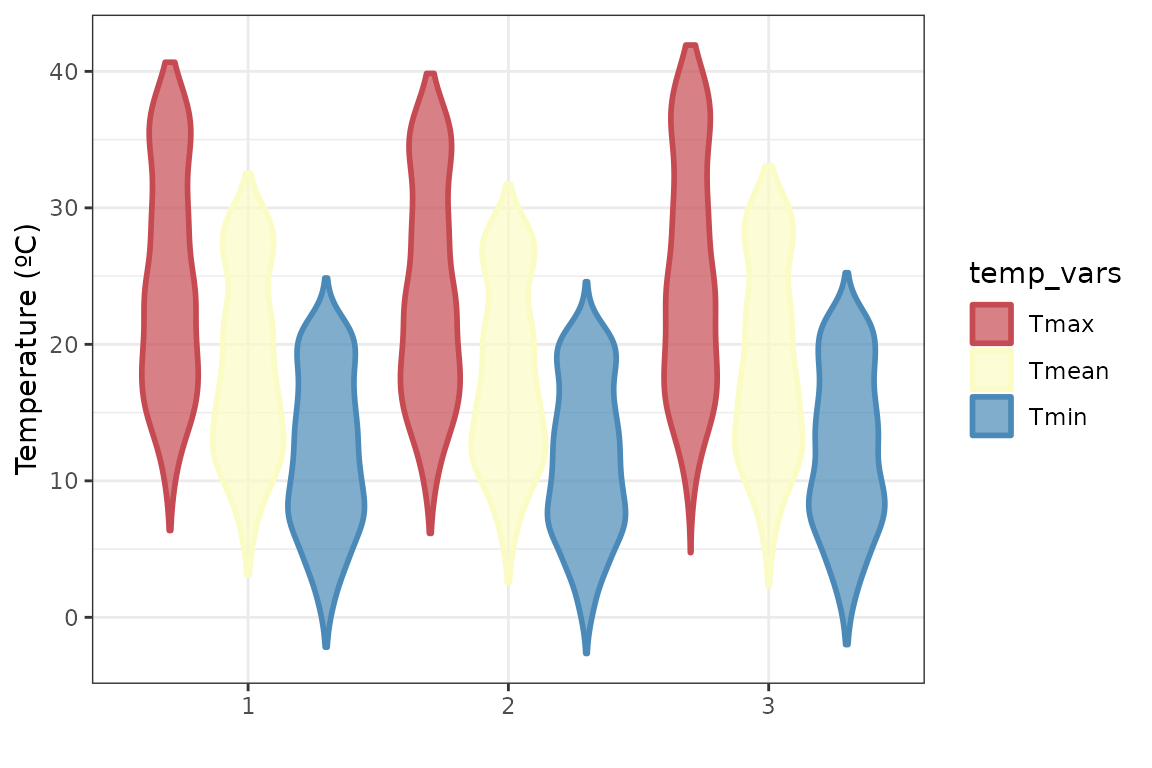
ggplot(temp_long, aes(x = date, y = temp_values, color = temp_vars)) +
  geom_point(alpha = .3) +
  scale_color_manual(name = "Variables",
                     values = c("#C54A52", "#FAFBC5", "#4B8AB8"),
                     guide = guide_legend(override.aes = list(alpha = 1))) +
  ylab("Temperature (ºC)") + xlab("Date") +
  theme_bw()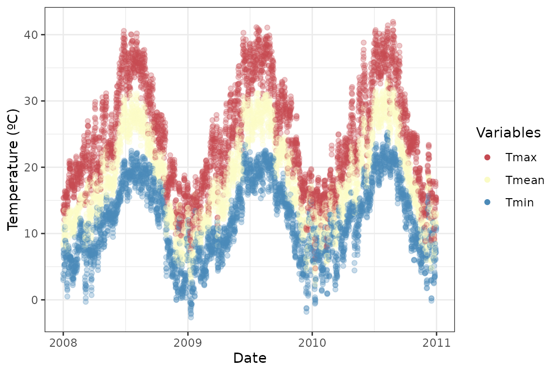
Example 2: Introducing coordinates as a matrix
{easyclimate} handles different input data, try now with matrices!
Here we are retrieving daily precipitation data for a single year (2008):
coords_mat <- as.matrix(coords)

Sys.time()
## [1] "2025-12-18 21:35:17 CET"

mat_prcp <- get_daily_climate(
  coords = coords_mat,
  period = 2008, # single year
  climatic_var = "Prcp"
)

Sys.time()
## [1] "2025-12-18 21:35:26 CET"

kable(head(mat_prcp))| ID_coords | lon | lat | date | Prcp |
|---|---|---|---|---|
| 1 | -5.780013 | 37.39833 | 2008-01-01 | 6.95 |
| 1 | -5.780013 | 37.39833 | 2008-01-02 | 25.34 |
| 1 | -5.780013 | 37.39833 | 2008-01-03 | 4.12 |
| 1 | -5.780013 | 37.39833 | 2008-01-04 | 0.00 |
| 1 | -5.780013 | 37.39833 | 2008-01-05 | 0.00 |
| 1 | -5.780013 | 37.39833 | 2008-01-06 | 0.00 |
mat_prcp <- mat_prcp |>
  mutate(
    date = as.Date(date),
    month = months(date),
    year = format(date, format = "%y")
  ) |>
  relocate(lon, lat, date, year, month, Prcp)

ggplot(mat_prcp, aes(x = date, y = Prcp, color = Prcp)) +
  geom_point() +
  scale_color_continuous(name = "Precipitation (mm)") +
  scale_y_continuous(expand = c(0, 0)) +
  coord_cartesian(ylim = c(0, 60)) +
  ylab("Daily precipitation (mm)") +
  xlab("Date") +
  theme_bw()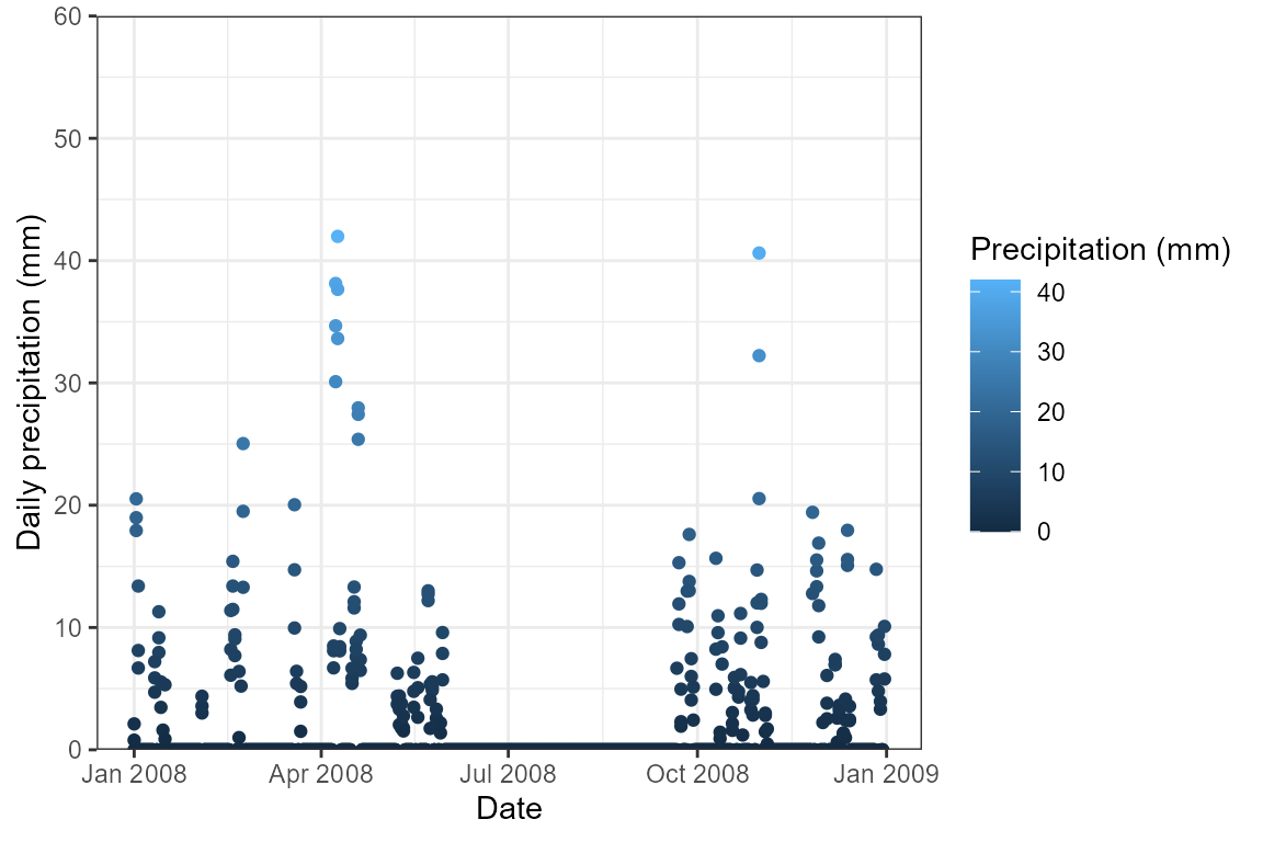
month_name <- format(ISOdate(2021, 1:12, 1), "%B")

mat_prcp |>
  mutate(month = factor(month, rev(month_name))) |>
  ggplot(aes(x = month, y = Prcp, color = month)) +
  geom_jitter(size = 2, alpha = .3, width = .3, show.legend = FALSE) +
  scale_y_continuous(expand = c(0, 0)) +
  coord_flip(ylim = c(0, 60)) +
  ylab("Daily precipitation (mm)") + xlab("Month") +
  theme_bw()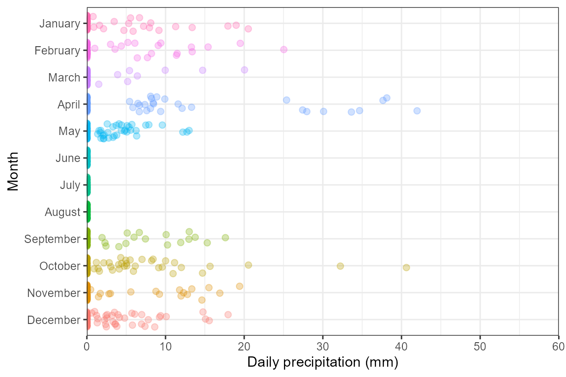
We can also retrieved monthly data using the same matrix of coordinates and add the average values to the previous plot:
Sys.time()
## [1] "2025-12-18 21:35:27 CET"

mat_monthly_prcp <- get_monthly_climate(
  coords = coords_mat,
  period = 2008, # single year
  climatic_var = "Prcp"
)

Sys.time()
## [1] "2025-12-18 21:35:28 CET"

kable(head(mat_monthly_prcp))| ID_coords | lon | lat | date | Prcp |
|---|---|---|---|---|
| 1 | -5.780013 | 37.39833 | 2008-01 | 47.50 |
| 1 | -5.780013 | 37.39833 | 2008-02 | 59.22 |
| 1 | -5.780013 | 37.39833 | 2008-03 | 14.89 |
| 1 | -5.780013 | 37.39833 | 2008-04 | 181.45 |
| 1 | -5.780013 | 37.39833 | 2008-05 | 51.06 |
| 1 | -5.780013 | 37.39833 | 2008-06 | 0.00 |
mat_monthly_prcp <- mat_monthly_prcp |>
  mutate(
    date = ym(date),
    month = month(date, label = TRUE),
    year = year(date)
  ) |>
  relocate(lon, lat, year, month, Prcp)


mat_monthly_prcp |>
  ggplot(aes(x = month, y = Prcp, color = month)) +
  geom_jitter(size = 2, alpha = .3, width = .3, show.legend = FALSE) +
  geom_point(
    aes(x = month, y = Prcp),
    size = 2
  ) +
  scale_y_continuous(expand = c(0, 0)) +
  coord_flip(ylim = c(0, 60)) +
  ylab("Monthly precipitation (mm)") + xlab("Month") +
  theme_bw() +
  theme(legend.position = "none")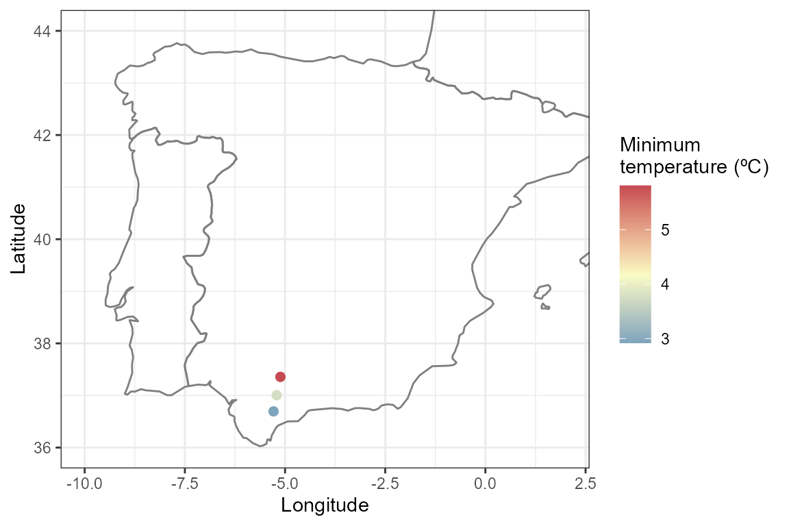
Example 3: Introducing coordinates as simple feature objects
Here we introduce coordinates as a sf object, and
retrieve minimum temperature for a single day (1 January 2001) and mean
temperature of a single year (2001):
library(sf)

coords_sf <- st_as_sf(
  coords,
  coords = c("lon", "lat")
  )

sf_tmin <- get_daily_climate(
  coords = coords_sf,
  period = "2001-01-01", # single day
  climatic_var = "Tmin"
  )

ggplot() +
  borders(regions = c("Spain", "Portugal", "France")) +
    geom_point(data = sf_tmin, aes(x = lon, y = lat, color = Tmin), size = 2) +
  coord_fixed(xlim = c(-10, 2), ylim = c(36, 44), ratio = 1.3) +
  scale_color_gradient2(name = "Minimum\ntemperature (ºC)",
                        low = "#4B8AB8", mid = "#FAFBC5", high = "#C54A52",
                        midpoint = mean(sf_tmin$Tmin)) +
    ylab("Latitude") +
  xlab("Longitude") +
  theme_bw()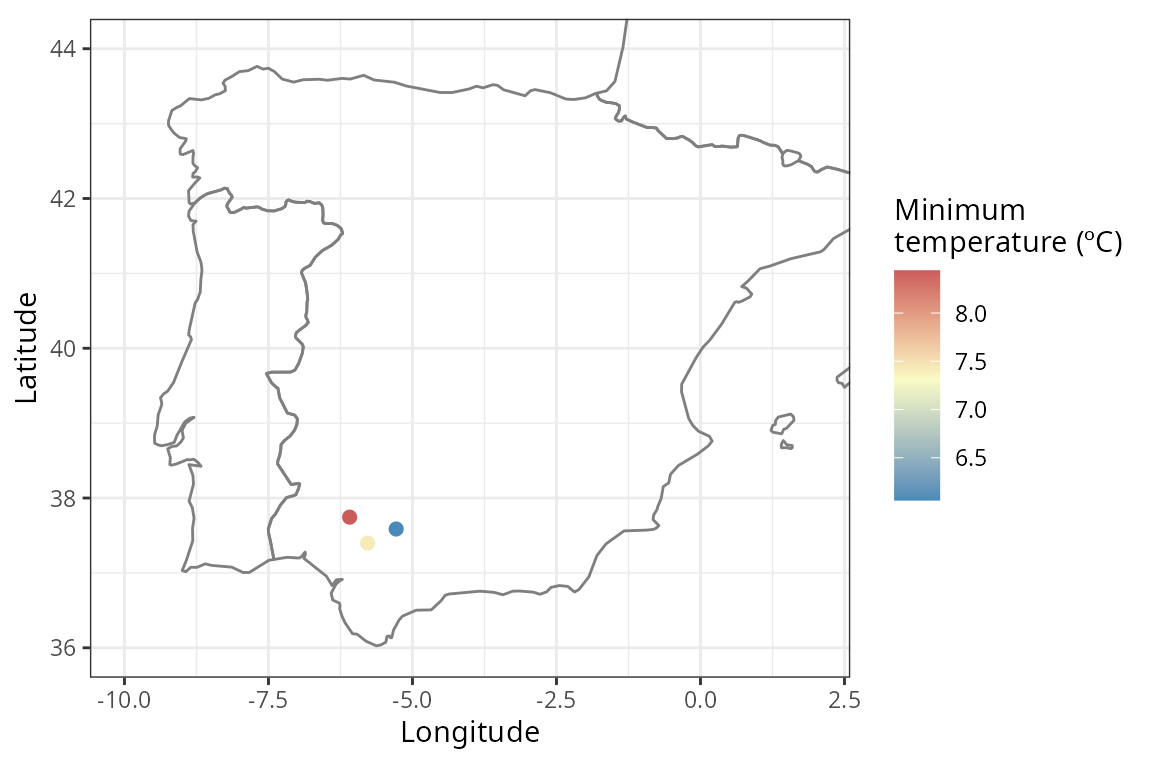
sf_tavg <- get_annual_climate(
  coords = coords_sf,
  period = 2001, # single year
  climatic_var = "Tavg"
  )

ggplot() +
  borders(regions = c("Spain", "Portugal", "France")) +
    geom_point(data = sf_tavg, aes(x = lon, y = lat, color = Tavg), size = 2) +
  coord_fixed(xlim = c(-10, 2), ylim = c(36, 44), ratio = 1.3) +
  scale_color_gradient2(name = "Mean\ntemperature (ºC)",
                        low = "#4B8AB8", mid = "#FAFBC5", high = "#C54A52",
                        midpoint = mean(sf_tavg$Tavg)) +
    ylab("Latitude") +
  xlab("Longitude") +
  theme_bw()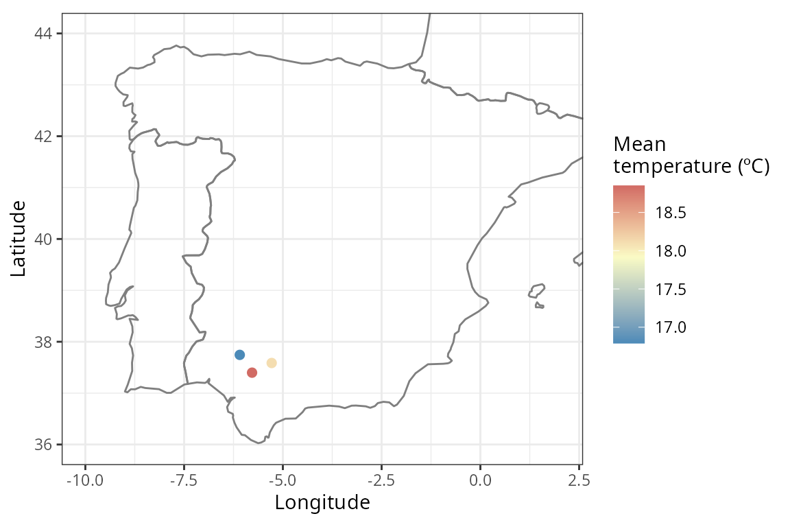
Learn more
Now you know how to obtain a data frame with different climatic variables with {easyclimate}, using point coordinates in different formats and downloading data for multiple locations and periods. Check out this other vignette if you need to extract the data of a complete area.